Why Machine Learning Outperforms Traditional Programming Methods
Traditional concepts of programming rely on either directly or indirectly leveraging the knowledge of human experts to determine the appropriate response to a given input. While these programs are ideal for handling limited, consistent input sets, they fall short in situations where the input data set is large, variable, or noisy – criteria which a large amount of real-world data meets. As an illustration, we can consider a 25×25 grid of black-and-white pixels as an input to handwriting recognition software; even in this simple case, there are 2625 possible input configurations!
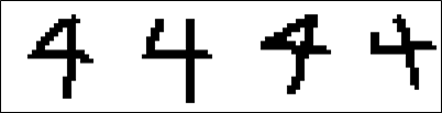 Programming an individual reaction to each of these input configurations would be impossible, not to mention tedious. Feasibly, one could attempt to program more general “rules” seeking to identify patterns in the input data instead of explicit input-output relations. However, variance in the input data (such as the shapes of individual letters or their location within the input grid) makes it difficult to identify a pattern or set of patterns that can consistently identify what symbol the input represents.
In an ideal scenario, we could ask the computer to program itself to recognize the symbols in the input pattern. Computers are, after all, much faster at manipulating data than a human could ever be – not to mention far less prone to boredom when performing repetitive tasks.
This idea of a computer programming itself (or, more frequently, adjusting the parameters of an existing program) forms the foundation of Machine Learning (ML). Notably, machine learning is distinct from the idea of Artificial Intelligence, although many concepts and techniques are shared across the two research fields.
The general concept of a learning machine has existed nearly as long as computing itself, having been originally proposed by Alan Turing in 1950. However, the abundance of data and computing power in the modern world has supercharged progress in the field of ML, transforming it from an academic research field into an engineering toolset with real-world applications across a wide spectrum of industries.
Given the ubiquity of machine learning in today’s connected world, many individuals who may not have previously learned about the topic are finding themselves in a situation where understanding the basics of ML would be beneficial. This article is intended for such individuals – either those who are starting on the road to deeper understanding, or those who only need to know the core concepts of the technology in order to understand how it could be useful to their specific situations.
What does “Machine Learning” actually mean?
Before reviewing the various means by which machine learning can be implemented, it is beneficial to have a concrete definition of what it means for a machine to learn.
First, however, a short note on terminology: While the term Machine Learning implicitly encompasses both hardware-based learning and software-based learning, all of the implementations and techniques discussed here are software-driven learning models. As such, the terms program, computer program, and machine may be used interchangeably to describe a given implementation, although program will be the preferred term in this article.
Informally, Machine Learning is a collection of tools, techniques and approaches that facilitate the creation of self-improving programs. It is important to note, however, that simply because a program is capable of self-improvement does not mean it is always actively improving. Many ML applications involve training a program to a given performance threshold and freezing the program at that point, preventing further changes to the program’s performance.
A more formal definition of machine learning was provided by Tom M. Mitchell in 1997, and remains widely quoted in the time since:
“A computer program is said to learn from experience E, with respect to some class of tasks T and performance measure P, if the program’s performance at tasks in T, as measured by P, improves with experience E”
For example, in the case of a handwriting recognition program, the task set T might be “classify handwritten letters from a series of images”, the performance measure P might be “percentage of letters correctly classified”, and E would be algorithm training using a dataset of letters tagged with the correct value.
In general, this definition can be used to highlight some of the key questions in the field of ML:
- What is the format of the experience E, and how is it obtained?
- How is the performance P of a program measured?
- What is the structure of the program?
- Which aspects of the program are fixed, and which may be changed by E?
- What is the procedure to internalize the experience E into the program’s behavior?
None of these questions has a single “right” answer. Instead, each represents a possible design decision that may be considered and adjusted to tailor an ML implementation.
Components of a Machine Learning Implementation
In order to expand on the discussion of what design decisions might go into the creation of an ML implementation, we can borrow some concepts from Systems Engineering. In particular, we can consider a generic implementation as a System of Systems containing a number of common functions along with the interfaces between them.
At a high level, any given ML implementation implements the following minimum set of functions:
- A learning function, which is responsible for parsing the experience dataset E and providing the necessary parameter adjustments to the internal model.
- An internal model, which in turn is comprised of subcomponents:
- A “static” structure representing those elements of the model that are fixed during design.
- A set of parameters which may be modified based on the learning function outputs
- A performance estimator, which implements the performance measurement P for internal and external use.
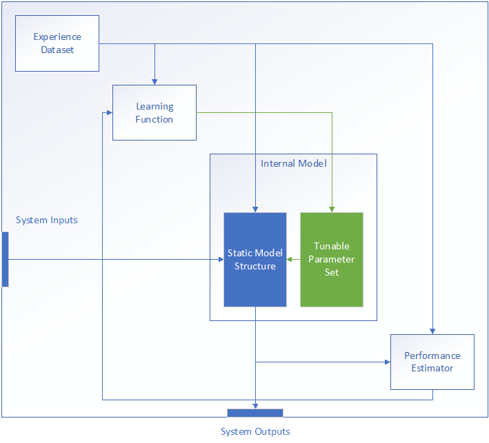 Additionally, the experience datasetE, also known as the training dataset, may also be considered either part of the system or as a subcomponent of the learning component. In either case, it is important to consider the training data during system design, specifically in regards to the required quantity, quality, and format necessary for the training operation to success.
While this generic model is necessarily quite simple, it is sufficient both to identify the key system components and the high-level interface considerations between each. In the next few sections, we will discuss the two components that form the core of any Machine Learning implementation: The internal model, and the learning function.
Types of Learning Function
Generally, there are four broad categories of learning function, classified based on the amount and type of feedback available to the system during training.
Supervised Learning
The first and most straightforward type of learning algorithm is a Supervised Learning (SL) algorithm. In this case, the system makes use of a “labeled” training dataset consisting of input-output pairs. Because each training input is explicitly associated to an expected output, the system has a known right answer for each input, and can calculate an error or cost function (closely related to the performance estimate P) representing the distance between the expected output value and the actual output.
SL algorithms are implemented for a wide range of problems, but they particularly excel at input identification problems such as image classification, information retrieval, and pattern recognition. More generally, any problem where it is possible to define a “correct” output for each input in a training set is a candidate for a SL approach.
While the exact method for adjusting the system parameters varies depending on the selected internal model, most SL algorithms utilize the same iterative optimization process to minimize the system error across the training dataset, as follows:
| Given a training dataset E consisting of inputs X and expected outputs Y, a cost function C(X), and an internal model M(X) with a corresponding set of tunable parameters A: |
| 1. Define a parameter η as the learning rate. This parameter represents a sort of “step size” in the optimization algorithm, with higher values of η resulting in larger changes to A with each iteration. |
| 2. Randomly divide E into N smaller datasets E1…EN, each containing n input/output pairs. For each subset, we label the corresponding input and output sets as XN and YN respectively. |
| 3. For each dataset Ei: |
| a. Process each input x in the set Xi through the internal model M(x) and calculate the cost function for that input, C(x) |
| b. Calculate the average cost function for Ei, |
| c. Using an optimization method such as gradient descent, identify the set of small parameter changes ∆A that results in the largest negative change in C(Ei), where the magnitude of ∆A is constrained by η. |
| d. Create a new set of parameters A = A + ∆A and apply them to the internal model. |
| 4. Optionally, return to step 2 and iterate across a new set of N random datasets. |
Although the general optimization flow is similar across SL methods, there are several intermediate steps that are highly method-specific – in particular, calculating ∆A in step 3c. As such, it may be beneficial to review the specific iterative flow of whatever method or methods are being considered for a given application.
In general, SL methods are the most commonly used learning method in Machine Learning, thanks in large part to the relatively straightforward optimization process they enable. This process has two particular benefits: First, while not necessarily completely intuitive, it is much simpler for a human to understand the optimization behavior than in some other learning paradigms. Second, the computational simplicity of the optimization process reduces the computing power required to train and implement the algorithm, lowering both the monetary cost of implementation and the time required.
The main drawback of SL methods, on the other hand, is the requirement for labeled data. Depending on the problem the ML implementation is working to solve, it may not be possible to sufficiently label a dataset, such as when trying to identify hidden patterns in data.
Even in cases where a labeled dataset is possible, there are potential problems. First, while a labeled dataset could be possible, one might not actually exist for the specific problem in question, potentially requiring human intervention or experimentation to manually compile and label the data. Second, the labels could be incomplete or inconsistent – for example, some photographs might be labeled as containing a bus but not labeled with the bicycles or cars that are also in the frame. On the opposite end, it is possible for a dataset to be overly labeled – while a photograph could be labeled with some of the objects in the image, attempting to label every object would result in an unusable mess of labels, and an ML implementation that believes that every possible input is “grass”.
Unsupervised Learning
In direct contrast to Supervised Learning, Unsupervised Learning (UL) algorithms work with untagged input data. These algorithms are therefore mostly unconcerned with outputting the right answer, as they have no indication as to what the right answer is.
Instead, UL algorithms generally operate through the principle of mimicry, seeking to generate an output that is similar to the given input. In principle, this act of mimicry is intended to mirror how humans (especially children) will mimic observed behavior such as speech as part of their learning process. Thus, during training, these algorithms will evaluate and optimize a cost function representing the difference between the algorithm’s output and the given input.
Most UL algorithms fall into one of two categories – either pattern identification, or so-called generative tasks. Pattern identification algorithms, as the name suggests, are generally used to identify unknown patterns or clusters within a dataset. As an example, a business analyst might employ a pattern identification network to identify unknown commonalities between customer groups in order to find a new marketing angle, or a medical researcher could test for common mutations in the genomes of cancer patients.
Generative tasks, on the other hand, deal with extending patterns identified within the input data in new ways. These tasks are, if given to humans, exercises in creativity such as image, speech or text generation. For example, the NVIDIA-created “AI Painting Demo” GauGAN2 generates images based off of any combination of text, segmentation, style preferences and/or user-generated images. Similarly, Sassbook is an AI story generator that generates short stories from a prompt and a genre selection. Figure 3 is an example short story generated by Sassbook from an appropriate prompt.
It is important to note that while these image- and text-generators are very impressive examples of what can be achieved with UL, they are also at the extreme cutting edge of such networks. For example, GauGAN2 was trained on a training dataset of 10 million images using one of the world’s most powerful supercomputers.
In general, while UL is capable of remarkable achievements, those achievements come at a cost. Part of this cost is in comprehensibility – most model architectures for UL are both large and difficult to understand, with many even employing random processes within the model in order to deliberately induce variance.
Another part of this cost is computational – these models are generally larger, harder to train, and more computationally complex than SL models. While part of this computational cost increase certainly resides in the fact that UL implementations are often called upon to handle more complex and open-ended problem sets than a typical SL implementation, it is also generally true that a UL implementation will require more training resources than a similarly-sized supervised model would.
Story generated by Sassbook from the prompt “I was reading an article on Machine Learning, when the most unexpected thing happened.”
I was reading an article on Machine Learning, when the most unexpected thing happened. The article was on artificial intelligence and a number of methods of solving problems. One was a kind of artificial human being. His name was Alan Turing. After all, he was the man who proved that not only did mathematical and scientific truth reside in numbers, they also came under the control of numbers. A number can be understood as a mathematical or scientific reality, or as an objective truth. Turing believed that if we could somehow use a computer to understand something about a certain problem, we would be able to solve it. He said that he believed we had not yet made the leap from the mathematical to the scientific and from mathematics to science, because we have had too many years of experience in mathematics and science to accept a new proposition as absolutely true.
Semi-Supervised Learning
Semi-Supervised Learning (SSL), as the name might suggest, occupies a middle ground between Supervised and Unsupervised Learning, and specifically concerns itself with situations where the input dataset is only partially labeled – in particular, where there is much more unlabeled data than there is labeled.
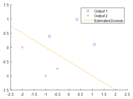 While the temptation exists to simply discard the unlabeled data from the learning set, this can often cause the model to be poorly fitted to the full dataset, and consequently to misassign inputs to the wrong output. For an example, consider the sparsely labeled data shown in Figure 4 – Given only these datapoints, the estimated division between Output 1 and Output 2 seems to be mostly linear.
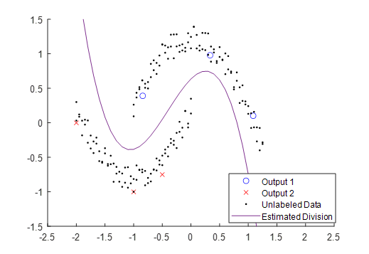
However, if we include the unlabeled inputs, a very different scenario takes shape, as seen in Figure 5. Even though these extra data points have a technically unknown output, we can see that the data forms two clearly-defined groupings. This observation, that sometimes unlabeled data can be grouped with nearby labeled data, informs many of the SSL approaches.
Specifically, SSL approaches make use of at least one of three basic assumptions:
- Points that fall close to each other in the input space are likely to share a label. This assumption, often referred to as a smoothness assumption, is also employed in supervised learning. In practice, this
 assumption creates a preference for decision boundaries to be both simple and to fall within relatively low-density regions, so as to avoid situations where points are close neighbors in input but categorized to different output classes.
 - Data tend to form clusters, and points within the same cluster are likely to share a label. This cluster assumption is a special-case restatement of the above smoothness assumption, and allows exploitation of the UL methods for identifying clusters and patterns.
- The data lie on or near one or more manifolds of much lower dimension than the input space. This manifold assumption is the least intuitive of the three, but generally refers to the idea that in an n dimensional input space, the position of datapoints may be approximated by a surface defined by n parameters, where n is much less than m. For example, the datapoints in Figure 5, while in a 2-dimensional space, approximately fall in the neighborhood of two one-dimensional parabolic manifolds.
Under these assumptions, SSL operates as something of a hybrid between the SL and UL approaches. For inputs which have a corresponding label, SSL will work to optimize the cost function at that input. However, for unlabeled data, SSL instead seeks to identify patterns within the data that might suggest the appropriate label for that input. Thus, an unlabeled point might be associated with another nearby point (whether labeled or not), with the algorithm building a chain of such associations until at least one of the associated points is labeled, at which point that label is propagated through to other associated points.
The SSL approach can also be generalized to cases where the labels in a dataset are generally considered suspect, the Weak Supervision (WS) problem (or, alternately, the SSL problem is one specific subset of the WS problem). In general, this problem occurs when the dataset has been insufficiently characterized for any of a number of reasons. In addition to the problem of sparse labeling addressed by SSL, one might have a situation where the available expertise is insufficient to confidently characterize data (particularly when working in complex fields such as cybersecurity or medicine), or a situation where an emerging problem must be analyzed and characterized as quickly as possible.
The WS approach addresses these uncertainties by introducing three general varieties of Weak Labels:
- Global statistics on groups of inputs – for example, we could be informed that ~50% of a given subset of training data should correspond to label A, without explicitly identifying which samples fall within that group.
- Weak classifiers – some or all of the labels in the training set may be weakly classified. This classification represents something of a catch-all for any number of error sources that could result in misclassification.
- Incomplete Annotation – This classification represents circumstances where some of the label data is missing from the training set, and represents a generalization of the SSL problem to include situations where label data may be corrupt or incomplete.
In general, the WS approach closely resembles the SSL approach, as might be expected. However, WS approaches will often attempt to optimize the input label map using a cost function and trial-based approach, performing a local optimization on the input map prior to employing the data for training.
Reinforcement Learning
Finally, the 4th and final category of ML approaches is Reinforcement Learning (RL), which represents something of a special case in the Machine Learning field. Like SSL, RL falls in the middle ground between SL and UL, although for different reasons. Recall that SL has full access to the expected output of all inputs in the training set, SSL has full access to the expected output of some inputs in the training set, and UL has no information about the quality of any output.
Instead of expected outputs, Reinforcement Learning instead provides the algorithm with a “reward” for a given input or action, without insight into how the reward is calculated. The overall objective of the system is then to maximize the total rewards collected by optimizing the system behavior.
Because the reward is calculated at the time an action is performed, reinforcement learning may be considered a “real-time” learning method. In contrast, the other learning models separate system operations into a training period and an operational period, with the system parameters being largely frozen during operation.
Thanks to their real-time nature, reinforcement methods are often employed in dynamic environments or, generally, where the specifics of the operating environment are unknown. This allows the system to react to changes in the environment or unanticipated inputs, whereas other models would react to an untrained input with truly unpredictable behavior.
In general, RL represents something of an edge case between several fields of study (Controls theory, Game theory, economics, information theory…), and as such has an extremely wide range of potential applications. RL implementations include robot control algorithms, traffic routing algorithms, and AI opponents for board games such as Go and Backgammon, to name only a few.
Because RL is such an outlier, many of the approaches it employs bear little resemblance to the Machine Learning techniques implemented in the other learning paradigms discussed, and as such are better suited to a general discussion of Controls theory, as that field can provide direct intuition into how RL works. However, recent research in the RL space has been focused on implementing variants of traditional Machine Learning techniques such as mimicry and deep neural networks, which we will discuss in the next section.
Models for Supervised Learning
Now that we have a basic understanding of the operation, performance and purpose of each of the four categories of learning approaches, we can move on to examine the models that those approaches employ. For simplicity, this discussion will mainly center around models employed in the Supervised Learning context, as these models provide context necessary to later understand Unsupervised Learning approaches. Additionally, the SL models presented here can be generalized to the SSL and WL cases discussed previously with minimal modification. This is the case because most of the required changes for SSL and WL are applied to the training dataset, not the model itself. Finally, we will leave aside RL models for the moment, since there is minimal overlap between the RL model set and those employed for other machine learning approaches.
Artificial Neural Networks
Of the model types commonly used for SL, the Artificial Neural Network (or simply “neural network”) is one of the most interesting, versatile, and frequently encountered. This model structure was deliberately designed to mimic the structure of the human brain, using configurable sets of Artificial Neurons. Thus, an explanation of the ANN begins with a discussion of what, exactly, an Artificial Neuron (from here referred to simply as a Neuron) is.
Neurons
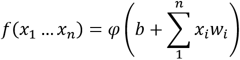
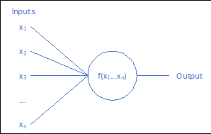 There are several varieties of neurons that can be employed in a neural network, but they all share a basic structure, as shown in Figure 6. Each neuron receives one or more inputs (either from the environment or from the preceding neuron layer) and performs a modified weighted sum calculation on those inputs, known as an activation function.
In addition to the inputs, a neuron’s behavior is dependent on three other terms: b, w1 and φ. The set of parameters represent the weights the neuron assigns to each input value (one for each of the n inputs), and directly affect the sensitivity of the neuron’s output to changes in that input. It is also possible to utilize negative weights, causing a neuron to become less likely to activate given a particular input.
The parameter is the neuron’s overall bias, indicating the general difficulty of activating that particular neuron, with higher values allowing the neuron to be activated at lower thresholds. As with the weights, a neuron’s bias can be negative, increasing the threshold required for activation.
Finally, φ is a special category of function known as a transfer function, and is selected based on what type of neuron is being implemented. Generally, there are three types of transfer function utilized in neural networks – the Step function, the Sigmoid function, and the Rectifier function. However, most modern neural networks employ either a sigmoid or rectifier function due to some convenient properties of those functions.
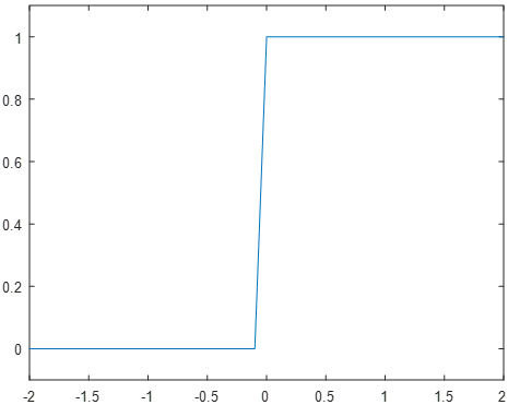 The Step function (sometimes also referred to as the Perceptron function after the first neural network) is the simplest of the three common functions, and was the first type of function implemented in neural networks. These neurons are either fully activated or fully deactivated, with no intermediate values, and are defined by the formula
![]()
Unfortunately, while the binary response of a step neuron helps both in intuition (a neuron is either firing or inactive, with no middle states) and in implementation (as the output is simply a one-bit value), it also introduces drawbacks that make it ill-suited to most machine learning applications. In particular, the step response does not communicate any information about the activation strength; an input of 0.01 produces the same response as an input of 10.
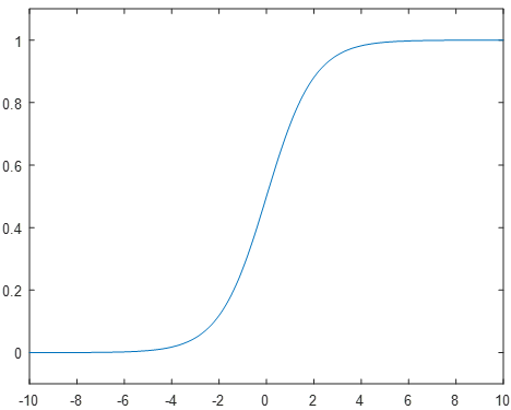 These drawbacks led to the adoption of the Sigmoid neuron, which converts the step function response to a smoothed curve around the input u=0. The sigmoid function is given by the formula
 ![]() and results in the plot shown in Figure 8.
and results in the plot shown in Figure 8.
Intuitively, the sigmoid function represents a smoothing of the step function used previously. At the extremes of -/+ infinity, the function approaches 0 and 1 respectively. However, in the neighborhood around a zero input, the function has a smooth curve where the step function has a discontinuous jump.
This smooth behavior is the critical feature of the sigmoid function, as it allows small changes in the system parameters to propagate through to the output. However, the non-binary response of the sigmoid neuron can complicate intuitions such as if the neuron is active or not. By convention, a sigmoid response above 0.5 is considered to be “active” when reading neuron outputs.
Finally, the Rectifier neuron is a relatively recent development, but it has become the most prevalent variety of neuron for new development. The rectifier is defined by the formula φ(u) = max (0,u), resulting in the plot in Figure 9.
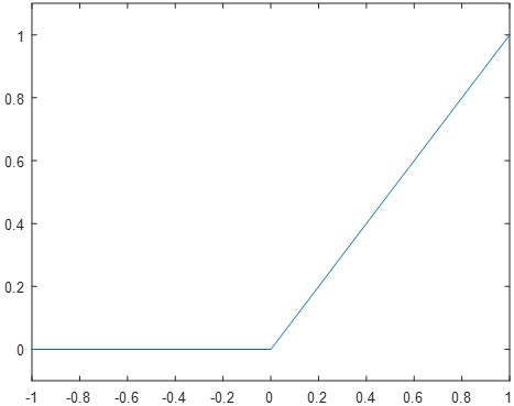 Notably, the rectifier function is the only one of the three functions presented that is not a normalizing function. Where the step function outputs either 0 or 1, and the sigmoid outputs a value somewhere between 0 and 1, the rectifier can have an output anywhere from 0 to positive infinity. In practice, the unbounded nature of the rectifier function is outweighed by other benefits, such as improved learning speeds and decreased computational complexity.
However, regardless of the specific activation function used, many of the underlying principles remain unchanged. Each of these functions takes a set of inputs x1…xn, multiplies them by a set of weights w1…wn, and adds a bias value b. As the weights and bias are adjustable and neuron-specific, this provides a set of n+1 tunable parameters that influence the neuron’s behavior.
Finally, for notational simplicity going forward, we can redefine the output ![]() of the ith neuron of the lth layer as
of the ith neuron of the lth layer as ![]() and is referred to as the weighted input for that neuron.
and is referred to as the weighted input for that neuron.
The Artificial Neural Network
While individual neurons are interesting on their own, their true value is in combining several neurons to form a network. In general, neural networks consist of 2 or more layers of neurons. Each neuron in a given layer receives inputs from the neurons in the previous layer, and provides an output either to the subsequent layer or to an observer. Simple networks may have only 2 or 3 layers, whereas more complicated networks may 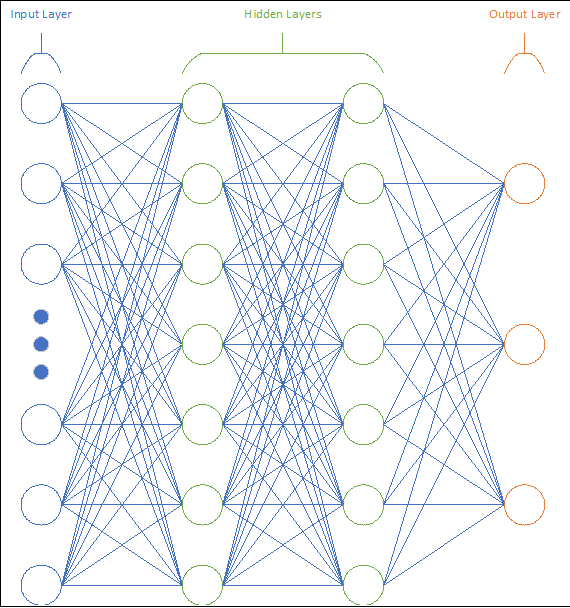 have dozens. These layers consist of an Input Layer, an Output Layer, and zero or more Hidden Layers. Figure 10 provides a visual representation of a general (4-layer) network.
The Input Layer, as the name suggests, is where the network receives input from outside interfaces, and consists of a number of neurons equal to the number of input values. For example, a simple handwriting recognition problem with a 25×25 pixel input grid would employ 625 input neurons. For other implementations such as speech recognition, the input layer could instead have one neuron for each sample in the audio file being fed in. Additionally, the input layer may be responsible for any data conditioning that is required, such as normalizing input values to between 0 and 1. However, such conditioning is not always required, and often the input neurons are simple pass-through functions for whatever data they are responsible for.
It is important to note that the Input Layer need not be composed of true neurons, especially if data conditioning is not required. Often, the input layer is a simple feed-through or storage of incoming data, with the neuron simply denoting which input variable is stored in that location.
The Output Layer is responsible for providing the network’s results to the user, whether that user is another computer program or a human observer. In the case of data identification tasks, this layer will typically have one neuron for each possible item it is identifying. Thus, for handwriting recognition without punctuation, the output layer might consist of 10 neurons for the digits 0…9, 26 lower-case letter neurons for a…z, and 26 upper-case neurons for A…Z for 62 total neurons.
Finally, the Hidden Layers are responsible for intermediate computation and pattern recognition. The exact number of hidden layers used for a given network is a somewhat subjective design decision, as is the number of neurons in each hidden layer. As such, it can be beneficial to develop an intuition as to what the hidden layers may be doing in a given network.
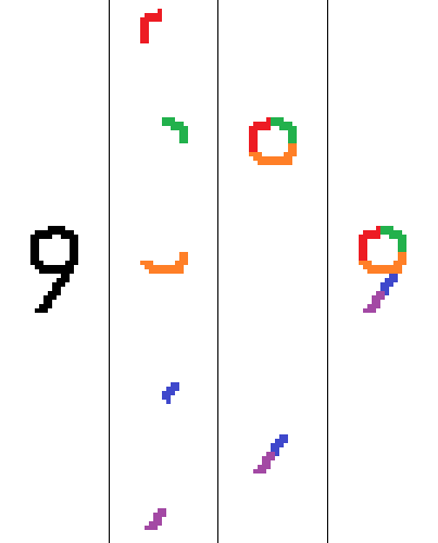 To understand hidden layers, it is helpful to consider what sub-components may be present in the dataset, and how they might be identified. For example, a handwriting recognition task might begin by identifying the small components that are present in an image (curves, lines). Once those components are identified, we could proceed by identifying larger sub-components such as loops and longer edges, and finally by identifying which outputs are most likely based on the specific sub-components identified, as shown in Figure 11. Similarly, for speech recognition one could start by identifying letter sounds, then syllables, then full words.
Each hidden layer present, then, roughly correlates to one layer of abstraction in the task at hand, with the number of neurons representing the number of possible variations at that level of abstraction. However, it is important to note that the sequences of abstraction that a human might implement may vary significantly from the trained network’s behavior; the network may instead identify other patterns which are less obvious to a human.
Advantages and Disadvantages of the Neural Network
In general, the neural network is an extremely versatile tool, or rather, family of tools. Specialized and optimized neural network variants have been developed for many different implementations, allowing an implementor to employ a pre-existing structure instead of iterating through the design process themselves. In particular, there are open-source implementations of high-performance visual processing, speech processing and text-to-speech processing networks available online, along with a myriad of other specialized implementations.
Unfortunately, there are several significant drawbacks to neural networks that prevent them from being a universal solution. In particular, neural networks are generally slow to fully train, often requiring multiple iterations across the training dataset. Additionally, the training speed for a general network decreases significantly as the number of hidden layers increases.
Adding to this difficulty, neural networks are computationally expensive to simulate in traditional digital computing hardware. While modern computers can somewhat “brute-force” this problem through sheer computational might, larger implementations still require hardware-based acceleration through an FPGA or GPU in order to train the network within any reasonable time frame. Alternately, there exist specialized processors known as Tensor Processing Units that are specifically optimized for neural network processing, but these units tend to be both rare and expensive.
Linear Regression
In contrast to the complexity of the Neural Network, Linear Regression(LR) is a very simple and straightforward model. Despite its simplicity, LR is one of the most widely-used models for Machine Learning, and in some ways represents the polar opposite approach to the neural network model.
LR belongs to the class of machine learning algorithms known, fittingly, as regression algorithms. These algorithms are generally used to predict a function’s behavior in a given region of the input space. Definitionally, for an n-dimensional input space x and associated output value y, the LR representation of a function is given by![]()
Where b0 is a bias coefficient, and b is a vector b1 … bn of weights for each variable in x. Training this model is then simply a matter of finding the coefficients and bias that minimize the cumulative error across the training data set. Fortunately, there exists the Ordinary Least Squares method to do exactly that.
Advantages and Disadvantages of Linear Regression
While the LR model is an exceedingly simple approximation of a function, in many applications it is good enough. Frequently, an LR model is the first model implemented in a given ML context, with more complex models being substituted if or when the first-order approximation provided by LR is no longer sufficient.
Fortunately, while inaccurate, LR is also very fast, whether in implementation, training or using the trained model to provide an approximation of the input function at a given point.
Where to go From Here
This article attempts to provide a high-level understanding of both Machine Learning as a whole, and two of the most common models used in the field. The foundation provided here should be sufficient to dive deeper into other aspects of ML depending on what specific interests or applications are paramount.
In general, ML is much easier to understand when working hands-on with practical examples. While some aspects are certainly mathematically daunting to look at (in particular the more detailed math involved in Neural Network training, as well as the specialized algorithms employed in Unsupervised Learning applications), it is much easier to develop a working understanding of what the math actually does when looking at a working example of the algorithm in code.
One resource I would particularly recommend for this sort of hands-on experience is TensorFlow, which encompasses an open-source collection of models, guides for getting started, and an open-source tool for working with ML. Matlab also has a robust ML toolkit, and the Matlab youtube channel contains tutorials on this and many other topics of interest.